You've entered your measurements or sales figures into a spreadsheet, added a chart, and found the trendline button. An equation appears, but you're not sure whether you selected the right columns, what the numbers mean, or whether a straight line belongs there at all.
Learning how to find the best fit line starts with a small calculation you can check yourself. We'll use a deliberately simple, hypothetical dataset, work through the arithmetic, and use the result to check Excel, Google Sheets, and Python.
Table of Contents
- Calculate the Best Fit Line by Hand
- Fit the Line in Excel, Google Sheets and Python
- Read Slope, Intercept and R-Squared Correctly
- Check the Scatter, Residuals and Failure Modes
- Apply Fit Lines to Ecommerce Sizing and Trends
- Choose the Right Tool for Your Fit
Calculate the Best Fit Line by Hand
Suppose your observations are (x = 1, 2, 3, 4, 5) and (y = 2, 3, 5, 4, 6). The question is: what straight line summarizes how (y) changes as (x) increases?
We want an equation in the form (hat y = mx + b), where (m) is the slope, (b) is the intercept, and (hat y), pronounced “y-hat,” is the predicted value. Actual measurements are (y); predictions are (hat y).
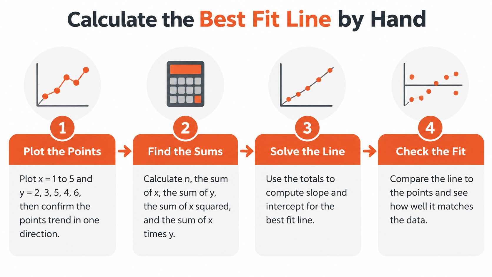
The graphic summarizes the workflow before the arithmetic.
Work from points to an equation
Plot the observations. Put (x) on the horizontal axis and (y) on the vertical axis. The points generally rise, despite a dip, so a rising straight line is a reasonable candidate.
Build the calculation columns. Multiply each row's (x) by its (y), then square each (x). Count the observations to get (n = 5), and add each column separately.
Worked example: sums, predictions and residuals
| x | y | x × y | x² | Predicted ŷ | Residual |
|---|---|---|---|---|---|
| 1 | 2 | 2 | 1 | 2.2 | −0.2 |
| 2 | 3 | 6 | 4 | 3.1 | −0.1 |
| 3 | 5 | 15 | 9 | 4.0 | 1.0 |
| 4 | 4 | 16 | 16 | 4.9 | −0.9 |
| 5 | 6 | 30 | 25 | 5.8 | 0.2 |
| Total | 20 | 69 | 55 | 20.0 | 0.0 |
The (x) column totals 15. The prediction and residual columns show the results you'll calculate after finding the equation.
- Calculate the slope. The symbol (Sigma) means “add the values,” so (Sigma xy) means add the row-by-row products, not multiply the column totals. Substitute the totals into:
[
m=frac{nSigma xy-(Sigma x)(Sigma y)}
{nSigma x^2-(Sigma x)^2}
=frac{5(69)-15(20)}{5(55)-225}
=frac{45}{50}=0.9
]
- Calculate the intercept. Use the slope and column totals to position the line vertically:
[
b=frac{Sigma y-mSigma x}{n}
=frac{20-0.9(15)}{5}
=frac{6.5}{5}=1.3
]
Write the fitted equation. Our result is (hat y = 0.9x + 1.3). These formulas select the ordinary least-squares line, which minimizes the total squared prediction errors.
Check the predictions. Substitute each (x) into the equation, then calculate residual (=y-hat y). For the first observation, the prediction is (0.9(1)+1.3=2.2), so the residual is (2-2.2=-0.2).
The residuals sum to zero, as they should for ordinary least squares with an intercept, allowing for rounding. That's a useful arithmetic check, although it doesn't prove that the relationship is straight.
Arithmetic check: Recheck the (x times y) column first if your answer differs. Adding products and multiplying sums are different operations.
For a bridge from handwritten calculations to plotted models, PlotStudio AI's regression code examples for research data provide a useful implementation reference.
Your plain-language reading is: each extra unit of (x) corresponds to a predicted increase of 0.9 units in (y), on average.
Fit the Line in Excel, Google Sheets and Python
Best fit line functions by tool
| Tool | Slope | Intercept | Show the fit visually |
|---|---|---|---|
| Excel | =SLOPE(known_y, known_x) |
=INTERCEPT(known_y, known_x) |
Scatter chart, Add Trendline, Display Equation and R-squared |
| Google Sheets | =SLOPE(data_y, data_x) |
=INTERCEPT(data_y, data_x) |
Insert chart, Customize, Series, Trendline, R-squared option |
| Python with NumPy | np.polyfit(x, y, 1)[0] |
np.polyfit(x, y, 1)[1] |
Matplotlib scatter plot with plt.plot(x, m*x + b) |
| Python with scikit-learn | model.coef_[0] |
model.intercept_ |
Plot predictions; model.score(X, y) returns R-squared |
Enter paired values in Excel and Sheets
Put the heading x in A1 and y in B1. Enter the example observations in A2:A6 and B2:B6, keeping each pair on the same row.
In Excel, enter =SLOPE(B2:B6,A2:A6) and =INTERCEPT(B2:B6,A2:A6) in separate cells. Notice that the y range comes first, even though the x column appears first in the worksheet.
Select both columns and insert an XY scatter chart, not a category-based line chart. Add a linear trendline, then enable the equation and R-squared display through the trendline options.
Google Sheets uses those same formulas. For its chart, choose Scatter chart, open Customize, expand Series, enable Trendline, choose Linear, and select the equation label and R-squared option.
Calculate and plot in Python
With NumPy and Matplotlib installed, the following commands reproduce the calculation. NumPy returns coefficients in descending powers, so the slope comes before the intercept.
import numpy as np
import matplotlib.pyplot as plt

x = np.array([1, 2, 3, 4, 5], dtype=float)
y = np.array([2, 3, 5, 4, 6], dtype=float)

m, b = np.polyfit(x, y, 1)
print(m, b)

plt.scatter(x, y, label="Observed")
plt.plot(x, m*x + b, label="Least-squares line")
plt.xlabel("x")
plt.ylabel("y")
plt.legend()
plt.show()
For a modeling pipeline, scikit-learn expects a feature matrix rather than a flat predictor array:
from sklearn.linear_model import LinearRegression

X = x.reshape(-1, 1)
model = LinearRegression().fit(X, y)
print(model.coef_[0], model.intercept_)
print(model.score(X, y))
Diagnose a mismatched answer
- Reversed inputs: Check the argument order in spreadsheet formulas.
- Text instead of numbers: Convert imported numeric text to numeric cells before fitting.
- Broken pairs: Remove incomplete observations as whole rows, rather than shifting either column independently.
- Different settings: Don't force the intercept to zero or select a polynomial trendline.
- Display rounding: Increase the equation's displayed decimal places before comparing coefficients.
Run the hypothetical example in any two tools. Both should return a slope of 0.9 and an intercept of 1.3, apart from tiny floating-point differences. A different result means the inputs or fitting settings differ, not that each tool has its own equally valid least-squares answer.
Read Slope, Intercept and R-Squared Correctly
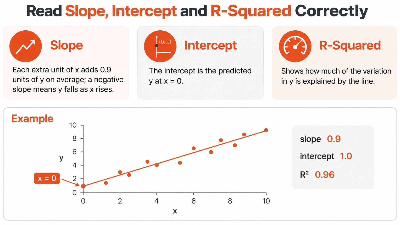
A fitted equation contains different kinds of information. The slope describes change, the intercept positions the line, and R-squared summarizes how closely the fitted values track variation in the observations.
The visual separates those roles.
Give the coefficients their units
Slope has units of y-units per x-unit. If your hypothetical (x) measures advertising spend in hundreds of dollars and (y) measures orders, the slope measures orders per additional hundred dollars, not orders per dollar.
A negative slope describes a decrease in predicted (y) as (x) rises. Neither sign establishes that changing (x) causes the change in (y).
The intercept is predicted (y) at (x=0). Its practical meaning depends on whether zero makes sense: predicting body weight at zero height isn't useful, even if an intercept helps fit the measured heights accurately.
Calculate what R-squared summarizes
For our hypothetical observations, the mean of (y) is (20/5=4). The total squared variation around that mean is:
[
(2-4)^2+(3-4)^2+(5-4)^2+(4-4)^2+(6-4)^2=10
]
Square the residuals from the table and add them:
[
(-0.2)^2+(-0.1)^2+1^2+(-0.9)^2+0.2^2=1.9
]
Therefore:
[
R^2=1-frac{text{sum of squared residuals}}
{text{total squared variation}}
=1-frac{1.9}{10}=0.81
]
This describes the share of observed variation accounted for by the fitted line relative to predicting the mean. It isn't the probability that the model is correct or a measure of causal certainty.
R-squared reference bands
| R-squared | What it suggests | What to check next |
|---|---|---|
| Near zero | Little improvement over predicting the mean | Whether the slope is useful and precisely estimated |
| Between the extremes | Some variation accounted for, with remaining scatter | Whether prediction errors meet the practical need |
| Near one | Observations lie close to their fitted values | Curvature, unusual points, leakage, and validation |
These are descriptive bands, not universal acceptance thresholds. A noisy behavioral outcome and a tightly controlled measurement process call for different expectations.
A high R-squared doesn't certify the model, and a low R-squared doesn't automatically make the slope useless.
A small slope can matter operationally, while a seemingly strong fit can still produce unacceptable individual prediction errors. Statistical uncertainty also needs separate assessment; R-squared alone doesn't tell you whether the slope is reliably distinguishable from no relationship.
Practice writing an interpretation with the variables, units, and R-squared. For this example: “Predicted (y) rises by 0.9 y-units per additional x-unit, and the fitted line has an R-squared of 0.81.”
Check the Scatter, Residuals and Failure Modes
Inspect the residual plot and influential observations before accepting the equation. Software can calculate a slope for data that a straight line describes poorly.
Best fit has a specific meaning here: the line minimizes the sum of squared vertical residuals. Squaring prevents positive and negative misses from canceling and gives larger misses more weight.
A residual plot helps you inspect what the equation leaves unexplained.

Look for patterns the line misses
Start with a scatter plot. A roughly straight cloud supports trying a linear model; a U-shaped cloud suggests that a single slope misses an important change in direction.
Say a retailer compares weekly advertising spend with weekly sales. A straight line might summarize a limited operating range, but promotional saturation could flatten the relationship at higher spending levels.
Then plot residuals against (x) or against fitted values. You're looking for a band around zero without a systematic shape.
- An arc: The model consistently misses in a curved pattern. Consider a scientifically or operationally meaningful transformation, or a curved model.
- A fan: The residual spread changes across the range. Predictions may be less precise at one end, and ordinary uncertainty estimates may need adjustment.
- Runs above and below zero: Time order, seasonality, or another omitted feature may matter.
- An isolated large miss: Check the original record, measurement process, and product category.
For apparel measurements, compare like with like before interpreting unusual points. A women's clothing size chart can help you keep chart conventions explicit, but nominal size labels aren't substitutes for measured garment dimensions.
Investigate influential observations fairly
A point far from the other (x) values can strongly affect the slope, especially when it also departs from the general trend. Refit with and without it as a sensitivity check, then report how the interpretation changes.
Don't delete a valid observation because the chart looks cleaner without it. Correct documented entry errors, and separate observations only when you have a defensible reason, such as a different garment construction or measurement method.
Before removing a point: Decide whether it's wrong, outside the intended population, or simply inconvenient. Those are different situations.
Keep prediction and inference within their limits
Predictions outside the measured (x) range are extrapolations. For demand, capacity, or customer behavior, a relationship that holds locally may flatten, reverse, or stop making practical sense beyond that range.
A tiny teaching dataset also can't establish stability. Adding another observation can change the estimate substantially, so don't mistake arithmetic precision for confidence about the wider population.
Shared seasonal changes can create an association without a direct causal connection. For example, weather might affect both activewear sales and advertising schedules, making spend and sales move together for reasons the simple model omits.
For conventional confidence statements, consider whether observations are independent, whether the conditional mean is modeled correctly, and whether residual spread is reasonably consistent. Small-sample inference may require additional distributional assumptions; repeated weekly observations deserve particular attention because neighboring weeks may be related.
If residuals show a pattern, the model needs more work. Treat the line as an association over the observed range, not proof that changing the predictor changes the outcome.
Apply Fit Lines to Ecommerce Sizing and Trends
A retailer can use a fit line to summarize sales direction or audit garment grading. These applications answer different questions, so keep their variables, units, and validation separate.
Inventory planning connects both kinds of analysis.

Separate a sales trend from a forecast
Fit monthly sales against a consecutive month index to summarize average change per month. Keep any projection short, identify the historical period used, and account for promotions, stockouts, and seasonal demand before treating it as a forecast.
Merchandising context matters too. A review of current fitness trends can suggest product categories to investigate, but a trend description isn't a numerical predictor until you define and measure it.
Audit sizing with measured garments
Define a comparable group. Select garments from the same style, construction, and intended fit, with repeated measurements across the available sizes. Record a clearly defined dimension, such as relaxed chest width measured flat.
Encode the size grade. Use an ordered numeric grade only when its spacing represents the intended grading steps. Don't assume that arbitrary labels or different brands share a common scale.
Fit dimensions to grades. Compare predicted dimensions with the actual garments and investigate systematic differences. Use production tolerances and fit requirements to judge acceptability, rather than turning residuals directly into shopper size bands.
Separate different constructions. Flag stretch fabrics, oversized cuts, and other distinct designs before combining measurements. They may need separate models rather than deletion as statistical outliers.
Test on held-out garments. Predict dimensions for garments you didn't use to fit the line, then measure them using the same procedure. This checks whether the grading relationship applies beyond the fitting sample.
A dimensional fit line is a quality-control tool, not a complete body-to-garment recommendation system. At Robosize, we match each product to the store's own size chart, support unlimited chart uploads, and give one precise size and fit recommendation for each specific garment.
For a separate storefront implementation reference, you can explore the Roval Components storefront project from Presidio. Keep storefront design decisions distinct from evidence that a sizing model predicts accurately.
The video offers an additional visual resource alongside the measurement workflow.
Choose the Right Tool for Your Fit
Choose the tool based on what you need to deliver, not on which interface looks most technical. A visible equation, an uncertainty estimate, and a production prediction pipeline are different deliverables.
Match the workflow to the decision
| Situation | Suitable starting point | Main reason |
|---|---|---|
| One-off homework or a quick check | Excel or Google Sheets | Easy inspection of cells, formulas, and charts |
| A regularly refreshed report | Spreadsheet formulas linked to a controlled data range | Repeatable updates without manual refitting |
| Coefficient inference | R's lm() or Python's statsmodels |
Model summaries, confidence intervals, and diagnostic tools |
| Predictions for new cases | Scikit-learn | Preprocessing pipelines and held-out evaluation |
For recurring spreadsheet reports, use structured tables or carefully maintained ranges. Make sure newly added rows enter both the formulas and the chart, and retain enough history to investigate unexpected changes.
For inference, R and statsmodels offer a clearer workflow than relying on a chart equation alone. Spreadsheet regression add-ins can also provide inferential output, but the basic SLOPE and INTERCEPT functions don't supply it.
For predictive work, reserve observations for testing before making model choices. With time-ordered sales records, preserve chronological order rather than randomly mixing future and past observations.
A shopper trying to search for a shirt needs a useful product-level answer, not a regression report. Keep the analytical checks behind the interface and present the resulting guidance in language shoppers understand.
Copy this final checklist
- Inputs: Paired observations are clean, and measurement units are recorded.
- Shape: The scatter supports the chosen model form.
- Diagnostics: Residual patterns and influential observations have been investigated.
- Interpretation: Coefficients and R-squared answer the actual business question.
- Validation: New-case predictions have been checked on appropriate held-out observations.
- Communication: The equation includes units and a clear statement of its intended range.
First run the teaching dataset in your chosen tool and verify its coefficients. Then replace it with your own observations, keeping the same checks rather than trusting the software output alone.
Robosize offers garment-specific size and fit recommendations matched to your store's own size charts. If your measurement analysis is ready to support shopper-facing guidance, visit Robosize to explore our virtual fitting room and request a live demo for your store.